Saturday, February 27, 2021

Chi-Square Tests of Independence testing using R ( Chi - Square Tests for two-way table )


             Chi-Square Tests of Independence

   ( Chi - Square Tests for two-way table )

  ===========================


For effective execution and analysis of the Chi-square test in R language we are going to do the following steps :


1) Step no.1
- We will create a vector in the following format

 data <- c(40,25,19,37,39)

 This "data" vector holds the data for all the students who are registered for the different classes in a school . These are 40 students in class 1 , 25 students for class 2 , 19 students for class 3 , 37 students for class 4 and 39 students for the class 5 .


2) Step no. 2 - In R we are going to evaluate whether the values as have been specified in the data variable object "data" are same in value and this equality condition is going to be tested in the NULLHypothesis for the test for evaluation of the data object .

 The Null Hypothesis and the Alternative Hypothesis for checking the validity of both the conditions can be stated and represented in the given manner with the null hypothesis being represented by the symbol (H0) and Null Hypothesis being represented by the symbol (H1) .


# H0 is the null hypothesis

H0 : p1 = p2 = p3 = p4 = p5


The alternative Hypothesis can be given in the alternate manner i.e,


# H1 is the alternative hypothesis

H1 : p1 != p2 != p3 != p4 !=p5


3) In the 3rd step , we will run the chi - square test over the function by calling the appropriate function for the evaluation of the same


·         chisq.test(data)


On the console one can see that the entire data item which had been fed to the prompt has been registed as a memory object . And when one wants to run the Chi-squared test upon the data item object , the values that come as a result of execution of the test are in the given format :


X-squared = 11.125, df = 4 , p-value - 0.02519


# from the given evaluation one can analyse with the help of the Chi-square table that the critical value which is also acronymised as (T-crit) is found to be as 9.488 with a degree of freedom for the data as 4 and alpha ( degree of significance is found out to be as 0.05 )

which can be found out from the p-value obtained after running the test is that we are basically not wrong in our assumption while framing the null and alternative hypothesis which means that the p-value for the evaluation is less than 0.025 which is less than the alpha value set for the test which is 0.05 then we can reject the null hypothesis as again stating .. we found out the P-value to be lesser than that of the Alpha set for the test.


 But had it been the case that the value of the alpha level had also been set at 0.25 then we would not have been at a position to reject the null hypothesis .


Conclusion and Verification


For the sake of analysing the obtained values if we are again running the chi-square test upon another pair of data in the given format .


data1 <- c(35,31,38,27,29)


 And again , we are running the chi-square test on these numbers in the "data1" vector , then the following results would be obtained .


> chisq.test(data1)


X-squared statistic is 2.5 , degrees of freedom is 4 , p-value is obtained as 0.644 .This means that since one is looking at the alpha value of 0.05 and the p-value is lying towards the left of the normal distribution line then we can say that the Null Hypothesis for the given set of values within the vector "data1" cannot be rejected .. I repeat , for the data values presented in the second vector item , the null hypothesis cannot be rejected .


 Again drawing a general conclusion from the experiment .. if we obtain the value of the p-value to be greater than that of the alpha value , then the null hypothesis cannot be rejected .


Friday, February 26, 2021

Keys of a Relational Database System ( detailed description with example on Primary Key Foreign Key , Candidate Key , Super Key )


·         One must have a way to specify how the tuples within a given relational table are distinguished from one another which is usually done with the help of attributes of the relation which means that the attribute values of a tuple must be as such so that they can uniquely identify any given tuple from a given database


·          In other words , no two tuples within a relation are allowed to have exactly the same value for all the attributes within a particular given relational table


·         So for the easier and effective identification of any unique tuple or row from a database the concept of recognition using "Superkey" was coined .


·         A Superkey is a set of one or more attributes that when taken collectively allows the identifier to uniquely identify a tuple within the relation .


·          Example :

   "customer_id" attribute of the relation Customer is sufficient to distinguish one customer tuple from another  tuple . Therefore , "customer_id" is a superkey in the relation .Similarly , the combination of the following  attributes "customer_name" and "customer_id" is a superkey for the relation "customer" . The "customer_name" attribute of "customer" is not a superkey because several people might have the same name .


·          The concept of superkey is not sufficient since a superkey may also contain extraneous attributes    within it .


·         If one is often interested in superkeys over a tuple for which no proper subset is a superkey then such minimal superkeys are called as "candidate keys"


·          In such a scenario , several distinct sets of attributes serve as a candidate key for a relation .Suppose a combination of "customer_name" and "customer_street" is sufficient to distinguish among members of the "customer" relation then both "customer_id" and {"customer_name" , " customer_street"} are called as "candidate keys"


·         Although the attributes "customer_id" and "customer_name" are together used to distinguish a "customer" tuple .. the combination does not form a candidate key since the attribute "customer_id" alone is a candidate key .


·         One can use the term "Primary Key" to denote a candidate key which is chosen by a database designer as the principal means of identifying the tuples within a Relation


·         A key ( whether primary , candidate or super) is a property of the entire relation rather than the individual tuples of the relation . Any two individual tuples in the relation are prohibited from having the same value upon the KEY attribute at any point of time . The designation of a Key represents a constraint in the real world  enterprise being modelled .


·          Candidate Keys must be chosen with utmost care . As noted , the name of person for being selected as a form of candidate Key is not completely sufficient since a situation may arise from the given scenario where multiple people with the same initials might happen and in such a case , all the data might be fetched with the same initials at any given point of time within the database . And as such duplicacy of value for such a candidate key is not entertained and as such any two tuples within the relation are prohibited from having the same value on the key attribute at the same point of time . The designation of a Key represents a constraint in the real world enterprise being modelled .


·          The Primary Key should be chosen in such a manner that its attribute values are never or rarely changed . For example , the address field of a person should not be part of the primary key , since the value is likely to change with the shifting of base / home from time to time . In the similar order , Social Security numbers of the dweller of any place can never change and remains the same from the time of birth to the time of death of the citizen . In the similar manner , Unique Identifiers generated by enterprises against any transaction are not likely to change and remain constant throughout and the given field could be considered as a primary key for a transaction relation .


·         Therefore , formally reiterating once again , if R could be considered as a Relation Schema and one would say that a subset K of R is a superkey for the table then the framer of the relational table restricts consideration to relations r(R) in which no two distinct tuples have the same values on all the attributes in K . This means that if tuple t1 and tuple t2 are in relation r and t1 != t2 then t1[K] != t2[K] .


·          A relation schema , say r1 may include among its attributes the primary key of another relation schema say r2 where this attribute is called as a foreign Key from relation r1 referencing the relation r2 . Here , the relation r2 is also called as the "referencing relation" of the the Foreign Key dependency and "r2" is called as the referenced relation of the foreign Key .


·         For example , the attribute branch_name in Account schema or relation is a foreign key . For example , the attribute "branch_name" in Account schema is a foreign key from Account schema referencing Branch schema since branch_name is the primary key of Branch Schema . In any database instance , given any tuple say "tn" from the "Account" relation there must be some tuple say "tn" from the "Account" relation there must be some tuple say "t2" in the branch relation such that the value of the branch_name attribute of tn is the same as the value of the            primary key that is "branch_name" of tb


 ·   Therefore , it is customary to list the primary key attributes of a relation schema before other attributes for example , the attribute branch_name of Branch Schema is listed first since it is the primary key


·          A database schema along with primary key and foreign key dependencies can be depicted pictorially as per the below given schema diagram . In the figure , a schema diagram for the banking enterprise has been depicted . Here , each relation appears as a Box with its attributes listed inside them and the name of the relation written above them . Hence , if there are primary key attributes , then a horizontal line crosses the box with the primary key attributes listed above the line in grey . Foreign key dependencies appear in the form of arrows from the foreign key attributes of the referencing relation to the primary key of the  referenced relation .


Many database systems provide design tools with a graphical user interface for the

 creation of schema diagrams .


Friday, February 19, 2021

Saving and Loading a DataFile in R Language


Manipulating Vector Objects in R Language


Manipulating Data Objects - A summary of involved steps in R


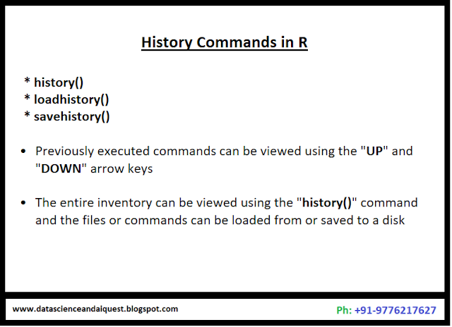
History Commands in R Language


Data Object Handling in R Language - Vectors , Dataframes ,Matrices and Lists


Commands for Finding Certain Data on a disk in R Language


Thursday, February 18, 2021

HDFS Design Goals in Big Data


Creating Lists using Range() function


Creating Lists using RANGE function


Python program to create lists with different types of elements


List Data Structure in Python


Lists and Tuples in Python


Lists and Tuples in Python


Lists and Tuples in Python


Functions in Python


Special Variable Name in Python


How to Install the Extra Packages of Windows


Sunday, February 14, 2021

Moments of Random Variable ( Mean and Standard Deviation Expression expressed in the form of score values )


Standardised Random Variables ( Mean / Standard Deviation )


Theorems on Variance with relation to Expectation and Mean


Variance and Standard Deviation in relation to Mathematical Expectation of a function variable - sample Representation in form of integral literals


Concept on Variance and Standard Deviation


Concept Theory on Variance and Standard Deviation in Probability and Statistics


Theorems on Mathematical Expectation and Probability Values


Functions of Random Variables with probability function


Definition of Mathematical Expectation of Values with an example


Example Question on Mathematical Expectation of Probability Values


Definition of Mathematical Expectation of Probabilities - Concept Theory expression

 part- 1


part-2


Concept Theory on Joint Distributions for two or more than two variables within a limit


A Graphical Representation of a Probability Distribution Function within limits - Example


Question to find the Distribution Function for Random Values with range limits


Example involving a constant value with a function lying within a specific range of values


Probability Distribution and Probability Function of a variable - Depition in form of integral limits and function of variable - an example


Depiction of Continuous Random Variables for a function of "X" where probability of value is in constraints


Distribution Function for Random Variables ( Graphical Representation with limit and range constraints ) - an example